For my MSc thesis I researched natural movements and the mechanical properties of the muscle. I combined these two topics to create a trajectory generating program for a differentially controlled robot. The program uses the two topics to control movement:
The biomimetic model generates a trajectory similair to natural movement. After this, the right parameters for the biomechanic model are estimated so that the biomechanic model generates a trajectory similair to the one found with the biomimetic model. For the estimation of the parameters, the BFGS algorithm from the GSL-library (GNU) is used.
To test the usage of the "twitch reponse" as an actuator model for a differentially controlled robot, a Java applet was programmed.
Make sure the GSL-library is correctly linked. I did this by opening Visual C++ (6.0, but 5.0 works similiar), click Tools->Options then select "include files" in the right menu and add the directory "\include\gsl" from the gsl library you dowloaded. It might help to copy gsl.dll and the libgsl.dll files to the directory where the compiled executable is. If this does not work , mail me: alex, subject "website", or leave a message in the weblog.
When a robot wants to move from A to B, it needs a motor command model to get there. In recent years, the type of navigation used in AI is reactive control. The steering behavior is directly coupled to its sensory input. Beceause there is always a time delay between this sensing and steering, a process called 'hunting' can occur. The figure below illustrates the hunting effect with a simple feedback control system like that from temparature control when using a thermostat.

This is why the model in my MSc thesis uses pro-active control. Pro-active control works like this:
Examples of pro-active control:
The jumping spider uses pro-active planning to jump to its prey :

The pro-active control model combines a biomimetic model and a biomechanic model. The model first generates a path with the biomimetic model. It then searches for a parametrisation for the biomechanic model, using the BFGS-algorithm. The result is a muscle-type of control to get from A to B with a differentially controlled robot.
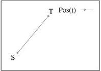
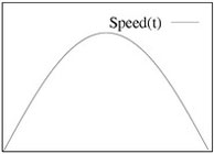
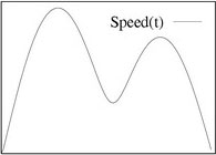
The trajectory that is generated with the biomimetic model is optimized for 'minimum jerk'. Minimum jerk is the change of acceleration. The quantity of 'jerk' is controlled by the spline that is used to construct the trajectory. Next to the shape of the trajectory, it is also important to look at the so called 'speed profile' of a trajectory. A smooth increase and decrease of speed during execution of the planned trajectory has several advantages:
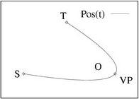
In the next figure movement with and without a via point (VP) are depicted(Where S is the Starting point and T is the Target). On the left side are the trajectories (x,y coordinates), on the right side are their speed profiles (y-axis:speed, x-axis:time). These trajectories were made using the biomimetic model.
The first model simulates a muscle twitch. A muscle can be described in mechanical terms. A.V.Hill (1938) was one of the first to research the mechanical properties of a muscle. He found out that a muscle can approximately be represented by the model in the picture below:
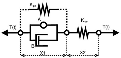
The components in the model are indicated by labels. T(t) stands for the tension or force. A.S. is the active
state or input to the muscle. B is the damping factor, represented by a capacitor. X_1, X_2 Are the contractile
element and the length of the series elastic element. K is the series elastic element.
The model enables simulation of a muscle reaction to neural input. Since we are investigating movements that involve
a planned trajectory, like the jumping spider's attack move, we look at the simplest form of muscle movement that
can accomplish this, which is the muscle twitch. When we solve Hill's model for a muscle twitch, we find the next
formula for the tension in a muscle during a twitch:
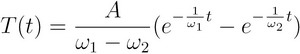
T(t) is the tension, A is the amplification. Omega-1 and omega-2 are the time-constants that determine the shape of the tension buildup and decay of a twitch response. In the picture below on can see a real twitch response at the left side, and two simulated responses at the right side (using different time constants causes the shape of the twitch response to change).
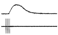
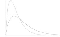
At the left side: twitch response of an isotonic contraction of a dorsal dilate muscle in the lobster in response to a 0.25 sec 30 Hz stimulus. At the right side two twitch responses using the formula from Hill's muscle model.
These twitch responses are used to differentially control a robot, where the right and left wheel are controlled by a different "twitch". This works as follows:

The resulting control type can be investigated in the Java applet.
The biomimetic model uses the same principles that Hogan & Flash found and described in their article "The coordination of arm movement: an
experimentally confirmed mathematical model." Journal of neuroscience, 5(7):1688-703 (1985).
The trajectory generated is actually a spline with 6 control points. The BFGS algorithm finds the right control points to generate a trajectory.
To get an idea of what a spline is, here is one:
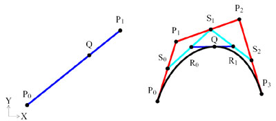
In the picture above: Left: linear spline, right: cubic spline. The path of point Q is the spline. This path is constructed by the control points. For the linear spline (left picture) these control points are P0, P1. In the case of the linear spline there is only one control point, Q, that travels from P0 to P1.The path of Q on the cubic is related to the traversal of the control points over the lines on which they are placed. Picture on the right hand: for the cubic spline the control points are P0, P1, P2, P3, S0, S1, S2, R0, R1. In the case of the cubic spline there are several control points traveling at the same time, eventually creating the path of Q. Two examples in the case of the cubic spline are S0 traveling from P0 to P1 and Q traveling from P0 to P3. All points that travel, travel in one second from their start point to their end point.
In the thesis, a more detailed explanation is given.